Steer-Prediction from Camera Images for Self Driving Car
NJIT CS782 Pattern Recognition & Applications Course Project
Source reference: Udacity’s Self-Driving Car Nanodegree project 3 - Behavioural Cloning
Abstract
The goal of this project is to train a deep learning model to predict steering angle for autonomous driving car in a simulator provided by Udacity. Using the vehicle’s camera images captured from the human driving demonstration, we train a deep neural network to predict the vehicle’s steering angle. The final trained model is evaluated both on the training track and an unseen testing track.
Overview
The project is consisted of the following modules:
- Project Requirement
- Setup and Environment
- Exploring the data
- Data Augmentation
- Deep Learning Model Design
- Model Training
- Performance & Evaluation
- Discussion
- Future Work
- Reference
Project Requirement
Deep learning model is trained only on Track 1 data. To assess the trained model’s performance, the car has to successfully drive by itself without getting off the road on Track 1 and drive the entire Track 2 without getting off the road.
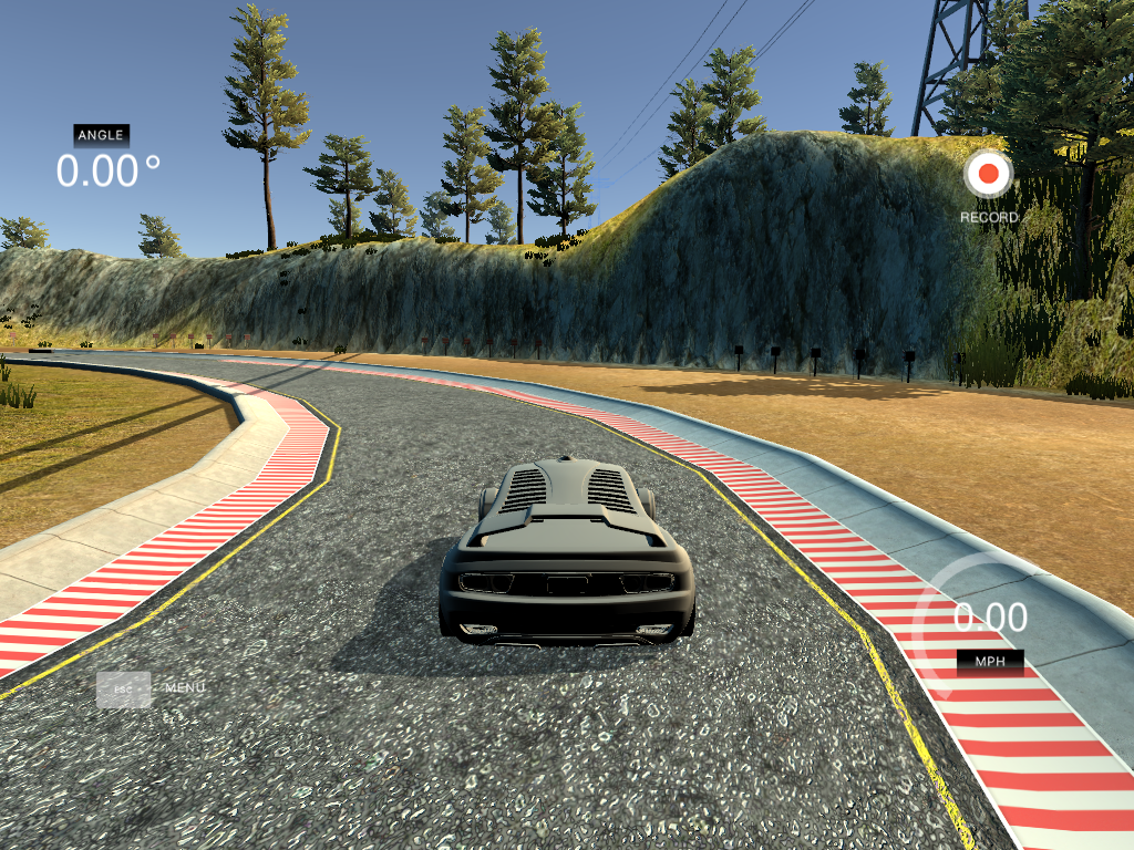
Track 1: flat road, mostly straight driving, occasionally sharp turns, bright day light.
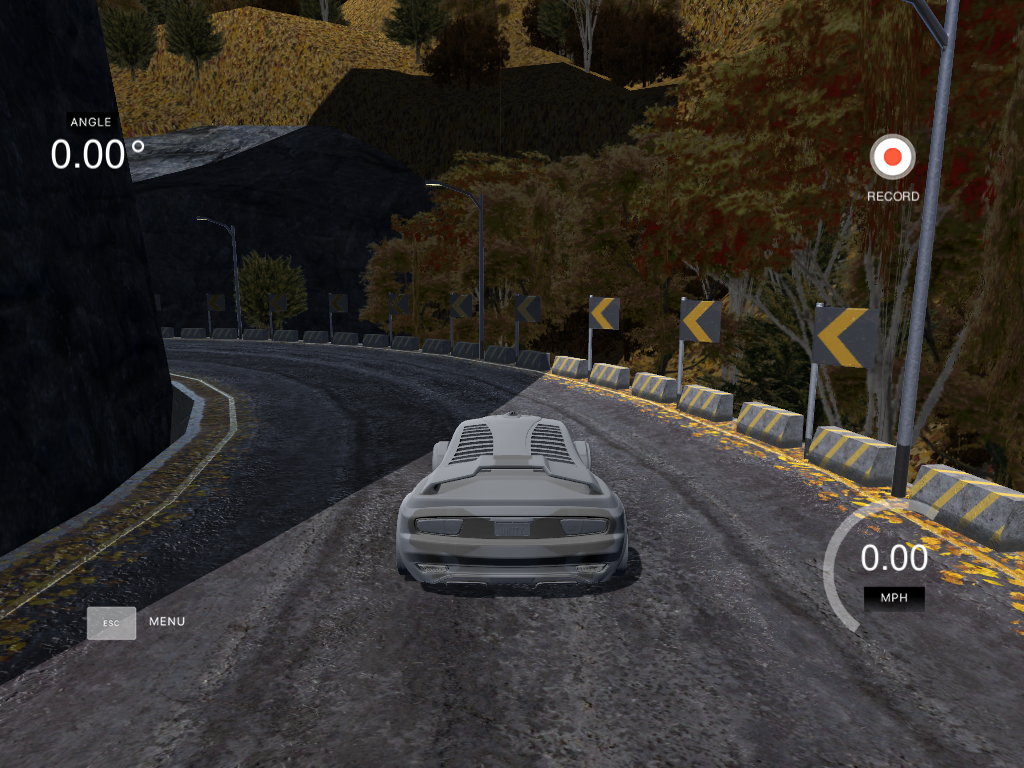
Track 2: hilly road, many light turns and sharp turns, dark environment, heavy shadows
Setup and Environment
Installation & Resources
- Python 3.5
- Anaconda Environment
- Udacity Car Simulator on Linux
- Udacity sample data
- Jupyter Notebook Download Both model training and drive programs are divided into steps with staged output and detailed explanation.
Files and Usage
-
autodrive35.yml: Anaconda Environment configuration file. -
p3-behavioural-cloning.ipynb: training program. -
model.json: saved training model. -
model.h5: saved training weights. -
drive.ipynb: program that takesmodel.jsonandmodel.h5as input to excute. -
To use:
- Start Simulator, pick track and choose Autonomous mode
- On
drive.ipynb, specify path tomodel.jsonandmodel.h5 - Run cell in
drive.ipynb
Quickstart
-
1. Control of the car is by using button on PC keyboard or joystick or game controller:
 accelerate
  brake
brake  steer left
  steer right
 - 2. Two driving modes:
- Training: User demonstrates driving on track
- Autonomous: Car drives itself by receiving commands from program
- 3. Collecting data:
- User drives on track 1 and collects data by recording the driving experience by toggle ON/OFF the recorder. Data is saved as frame images and a driving log which shows the location of the images, steering angle, throttle, speed, etc. Training images were sampled at 10 Hz.
- Another option is trying on Udacity data sample.
Exploring the data
Data Format/Component
- Camera Frame:
- There are 3 cameras on the car which shows left, center and right images for each steering angle.

- Driving Log:
- After recording and save data, the simulator saves all the frame images in
IMGfolder and produces adriving_log.csvfile which containts all the information needed for data preparation such as path to images folder, steering angle at each frame, throttle, brake and speed values.
- After recording and save data, the simulator saves all the frame images in

In this project, we only need to predict steering angle. So we will ignore throttle, brake and speed information.
Smooth Steering Angle
Since driving data was collected using keyboard inputs, the input time-series is very choppy. To smooth the data, I used a simple moving average, with a window of 3 time units (i.e. 0.3 seconds). Below is a plot of the raw and smoothed steering angle over time, for a random section in my normal driving data:

Data Balancing
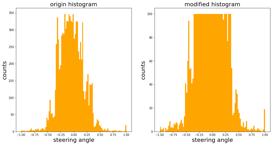
Collected data is not balanced, we can see the steering angle historgram as shown below and data balancing is a crucial step for network to have good performance!
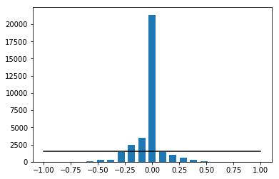
In order to balance the data, first, we can draw a histogram to see which steering angle ranges are most dominating in the sample space(high bins in the drawing). Secondly, we can calculate average samples per bin(as average_samples_per_bin) by dividing the total number of samples by the number of bins(200). Thirdly, we can determine keep probability for each bin: if the number of samples in a bin is below average_samples_per_bin, keep all; otherwise, the keep probability is set proportional to the number of samples above the average, in order to bring the number of samples for that bin down to the average.
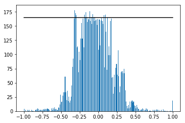
We can see from above figure, still, most of the steer angles are around the center(0 degree). There is very low probability that we will pick up the large angle portion samples. Thus, we need to further reduce the number of high bins, and this is done by function balance_data(). I use this function to bring the number of samples in each bin to 100 at most among 100 bins. After these steps, I had 4417 number of data points. The results are shown below:
Data Augmentation
Apparently, 4417 samples is a small training set, but we can apply some tricks that are already widly used for image classification to generate more samples:

reference: Building powerful image classification models using very little data
Here I chose 4 methods which are relevant to this project:
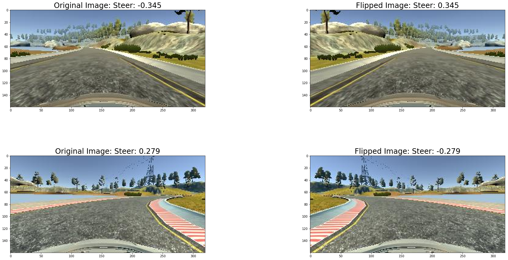
- Image Flipping: In track 1, most of the turns are left turns, so I flipped images and angles. As a result, the network would learn both left and right turns properly. Here are two images that have then been flipped:
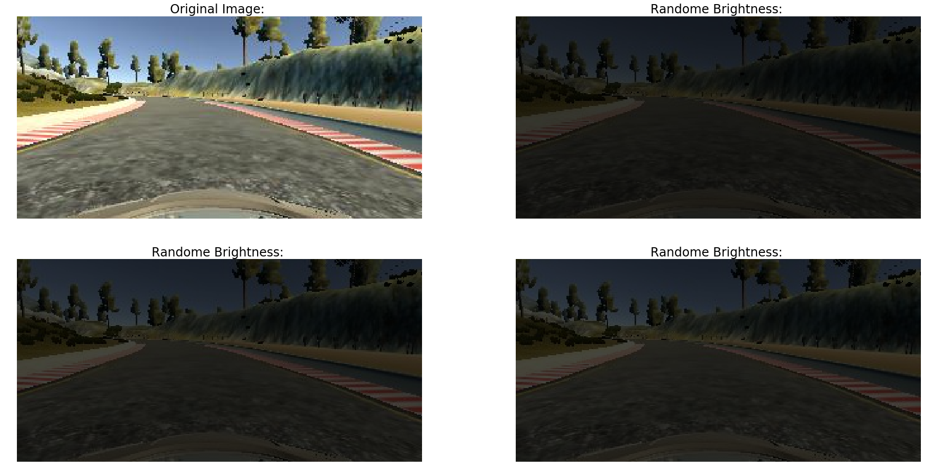
- Brightness Augmentation: In order to learn a more general model, I randomly changed the image’s brightness in HSV space(function brightness_change):
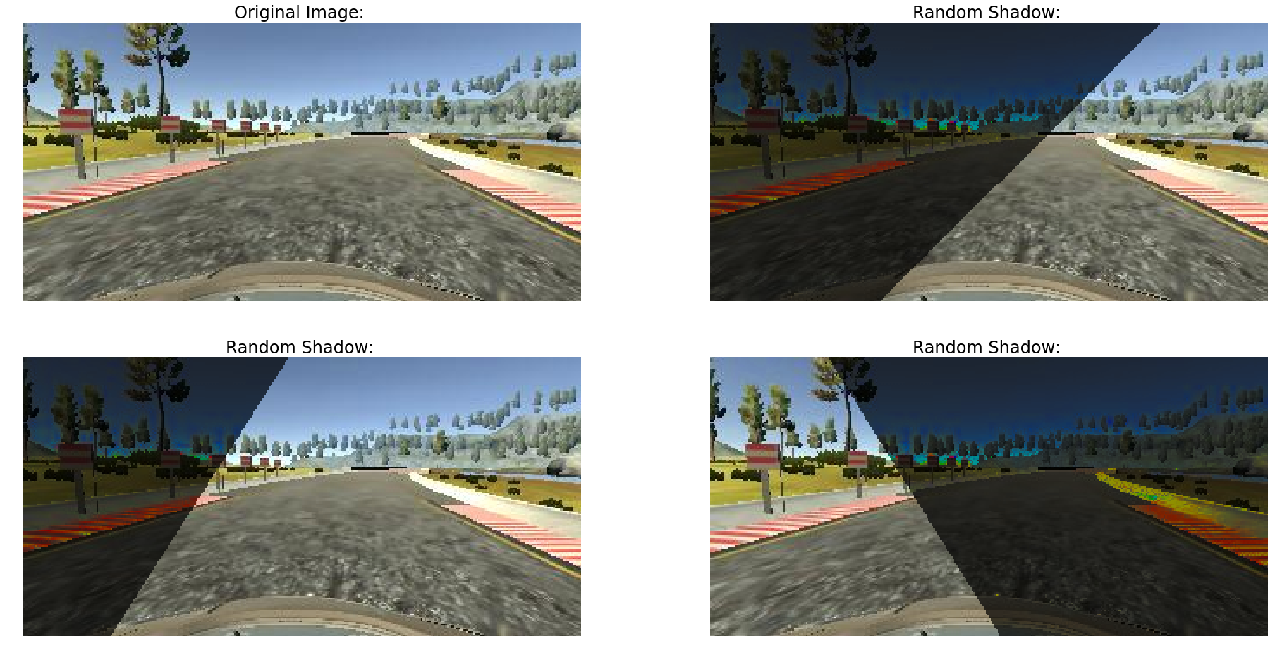
- Shadow augmentation: To deal with tree, building or other object shadow on the road, random shadows are cast across the image. This is implemented by choosing random points and shading all points on one side (chosen randomly) of the image(function add_random_shadow):
- Horizontal and vertical shifts: To simulate the effect of car being at different positions (driving up or down the slope) on the road, we can shift the camera images horizontally (vertically) and add an offset corresponding to the steering angle. We added 0.004 steering angle units per pixel shift to the right, and subtracted 0.004 steering angle units per pixel shift to the left(function trans_image):
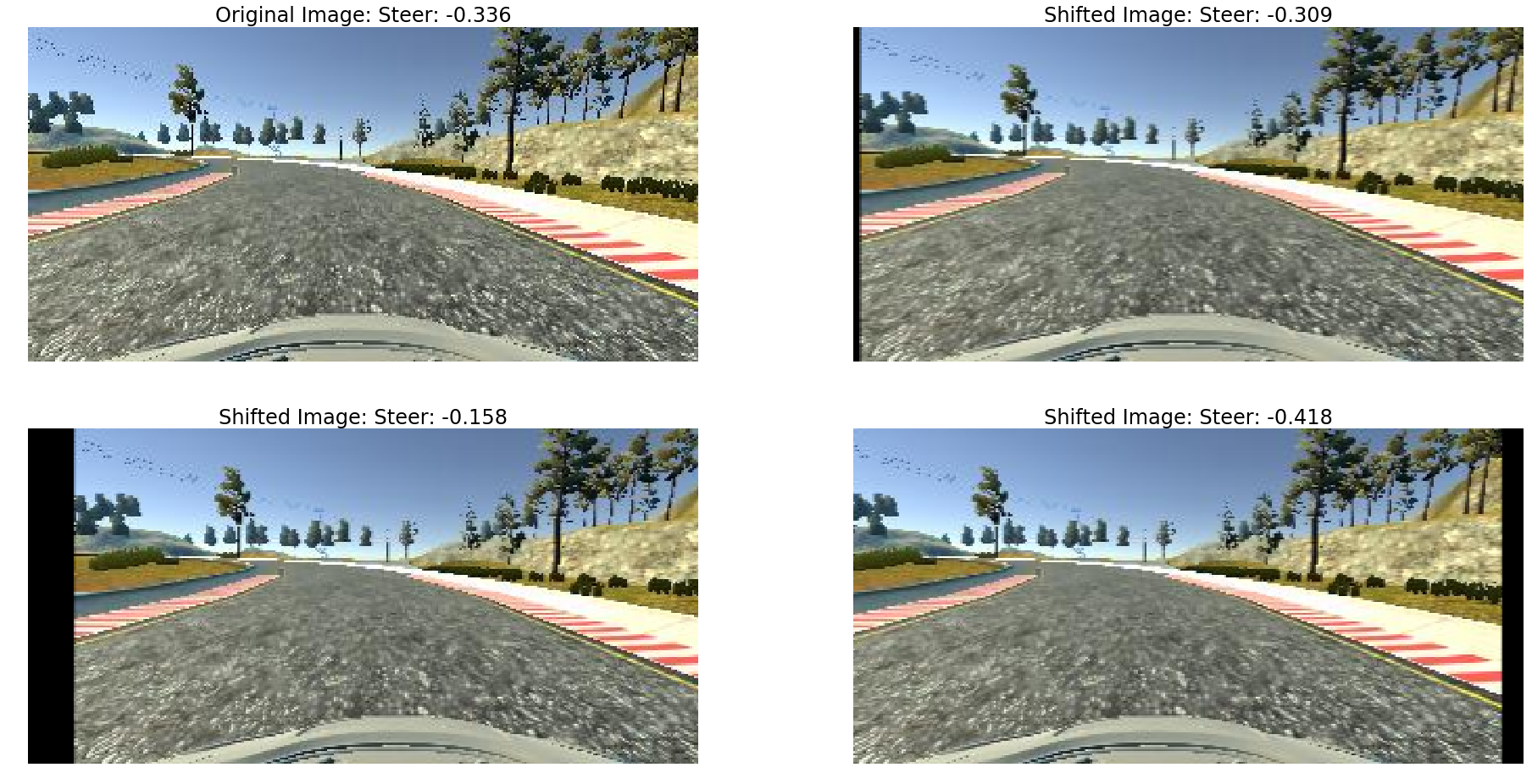
Note: I only use data augmentation in training phase, thus for each data point(sample), I will select FOUR images: center, left, right and horizontal shifting on center image. Then these four images then go through data augmentation process: Image Flipping, Brightness Augmentation and Shadow Augmentation. In validation phase, only center images with simulator provided angle labels are used to guarantee accuracy.
To summary, we will have approximately 13,251 data points available for training, and total number of images is around 53,004 with augmentation.
Deep Learning Model Design
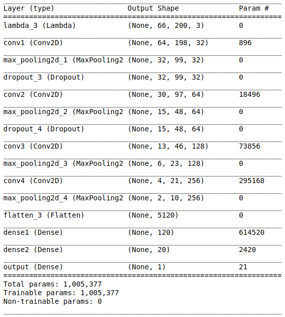
To find the best fitting model, I experimented with 3 existing models:
All of three models I explored share the following design structure:
- First phrase:
- Normalize input image data to -1 to 1 or -0.5 to 0.5 range
- Color space conversion layer(Optional): enable the model to select between 3 color channels
- Second phrase:
-
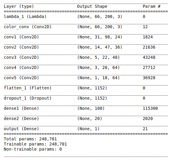
Convolution Layerare applied with 5x5 filter size but the depth increases at each layer such as 24, 36, 48. Then, 2 convolution layers are applied with 3x3 filter size and 64 depth. -
Maxpooling Layercan also be used at choice to decrease the input size -
ReLU/ELU Activationis applied following every convolution layer
-
- Third phrase:
-
Dense Layer– Output from previous layer are flatten. Then dense to 1 output (steering angle) via a few progressive layers, for example from 100 to 20 to 1. At each dense layer except the last, 10% to 50% (at your choice) Dropout is also applied to avoid overfitting. L2 weight regularization is recommended in every convolution and dense layer to produce a smoother driving performance. After many trial and error, 0.001 produce best peformance for this model. -
Dropout Layer– To avoid overfitting, Dropout with certain percentage can be added before or after the dense layer.
-
- Fourth phrase:
- Optimizer(Learning Rate): Adam optimizer is suitable for this project, which can automatically adjust the learning rate. It is set with default value 0.001, but 0.0001 learning rate is recommended to avoid too aggressive error descedent and produce a smoother ride. Therefore, 0.0001 learning rate is selected.
- Loss Function (or objective function, or optimization score function): Mean Squared Error(MSE) is used to measure the deviations of model predicted steering angle to human driver’s steering angle.
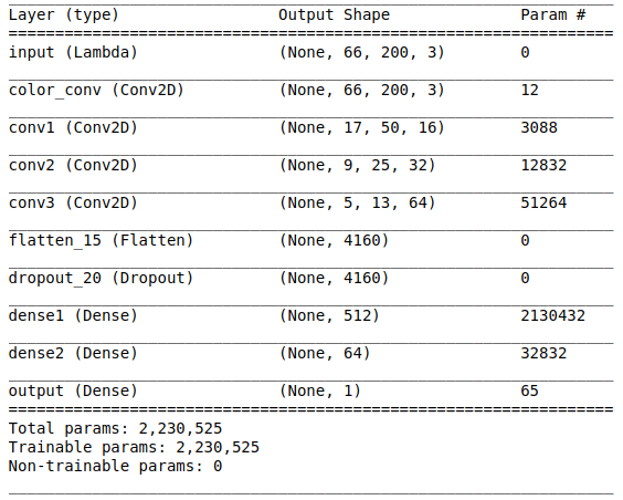
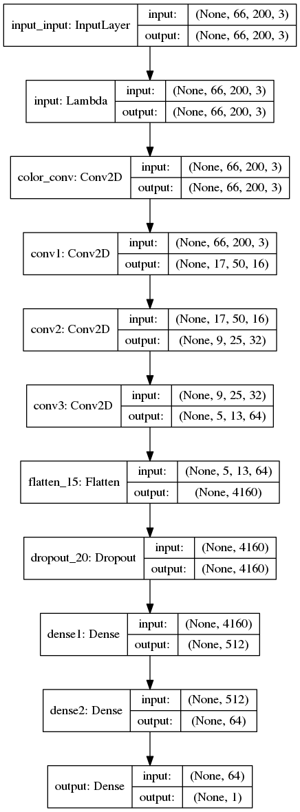
Structure summary of above three models implemented with Keras:
1. NVIDIA Model
|Model | Model Layer Details | |————————-|————————-|

2. Comma.ai Model
|Model | Model Layer Details | |————————-|————————-|
3. Simplified VGG Net - with configuration A
|Model | Model Layer Details | |————————-|————————-|

Model Training
Image Crop
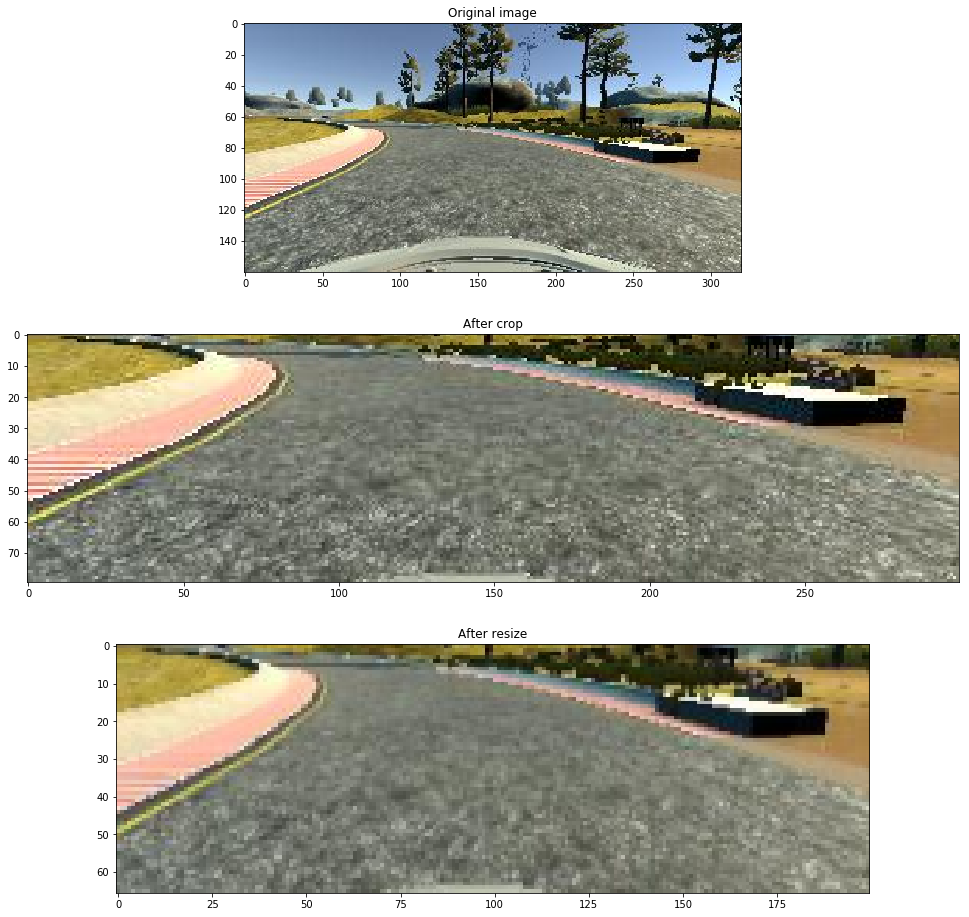
- To help the system avoid learning other part of the image but only the track, we can crop the up part (sky) and bottom part (front part of the car deck) out of the image. Original image size (160x320), after cropping 60px on top and 20px on the bottom, and 10px from left and right, the new image size is (80x300).
- To help running a smaller training model, images are scaled to size (66x200) from cropped size (80x300).
Convert to YUV color channels
The input image is split into YUV planes and passed to the network (reference the NVIDIA paper). 
Training and Validation
Central images and steering angles are shuffle and split into 70/30 for Training/Validation using shuffle & train_test_split from sklearn. Finally randomly shuffled the data set and put 30% of the data into a validation set.
Recovery
In general sense, driving behavior can be trained using the central images because we always look ahead when driving. Driving is mostly straight driving as well or small adjustment to turn the car unless there is a sharp turn. Below is the plot of steering angle on track 1 from Udacity data.
But from inutition, if our car goes off lane (for example, distraction during text and drive), we can adjust it back on track right away. The machine doesn’t have this intuition, so once it goes off road it would be hard to recover. To teach the machine this kind of recovery knowledge, we have to show it the scenarios. Hence, we use left and right camera images. Udacity gives out a great hint how to apply this method.
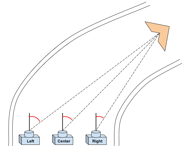
In the simulator, you can weave all over the road and turn recording on and off. In a real car, however, that’s not really possible. At least not legally. So in a real car, we’ll have multiple cameras on the vehicle, and we’ll map recovery paths from each camera. For example, if you train the model to associate a given image from the center camera with a left turn, then you could also train the model to associate the corresponding image from the left camera with a somewhat softer left turn. And you could train the model to associate the corresponding image from the right camera with an even harder left turn.
Steering Angle Correction
When we process the left and right camera, we add corrections (+0.25 or -0.25) for their steering angles because we only know the ground-truth steering angle for the center camera (as given by Udacity simulator). Therefore, it may introduce some small errors for the steering angles of left and right images.
The chosen left/right images and adjusted angles are then added into driving left or driving right lists. Here is the logic: adjustment_angle = 0.25
- Left turn(negative angle): + adjustment_angle on left image, - adjustment_angle on right image
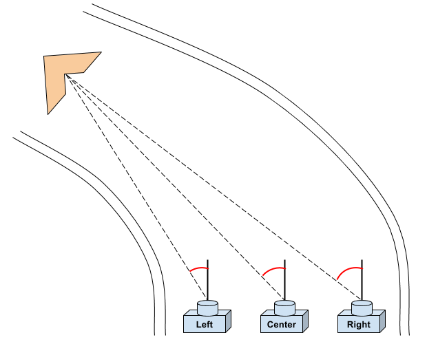
- Right turn(positive angle): + adjustment_angle on left image, - adjustment_angle on right image
Generators
There are two generators in this project. Training generator is to generate samples per batches to feed into fit_generator(). fit_generator() is used to fit the training model. At each batch, random samples are picked, applied augmentation and preprocessing . So training samples feeding into model is always different. Validation generator is also to feed random samples in batches for validation, unlike training generator, only central images are used here and only proprocessing is applied.
| Model | # of Epoch | Batch Size | Average Time per Epoch(in second) |
|---|---|---|---|
| NVIDIA | 20 | 64 | 54 |
| Comma.ai | 20 | 64 | 61 |
| Simplified VGG Net-A | 20 | 32 | 102 |
Performance & Evaluation
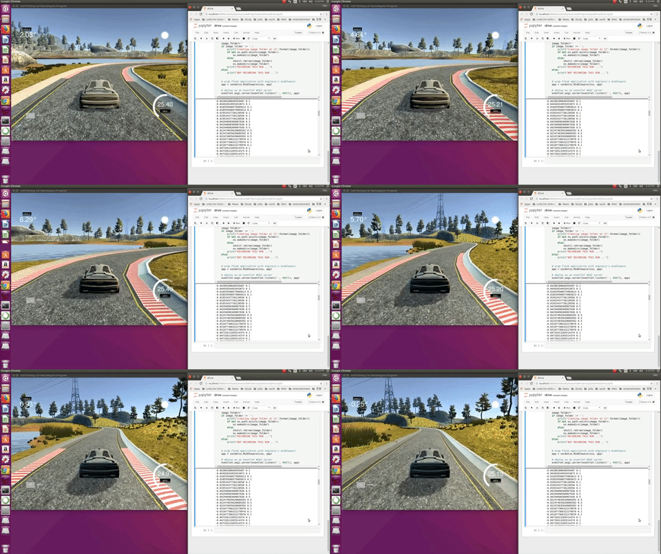
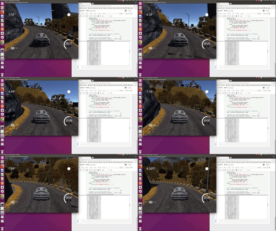
1. NVIDIA Model
2. Comma.ai Model
[Youtube link]
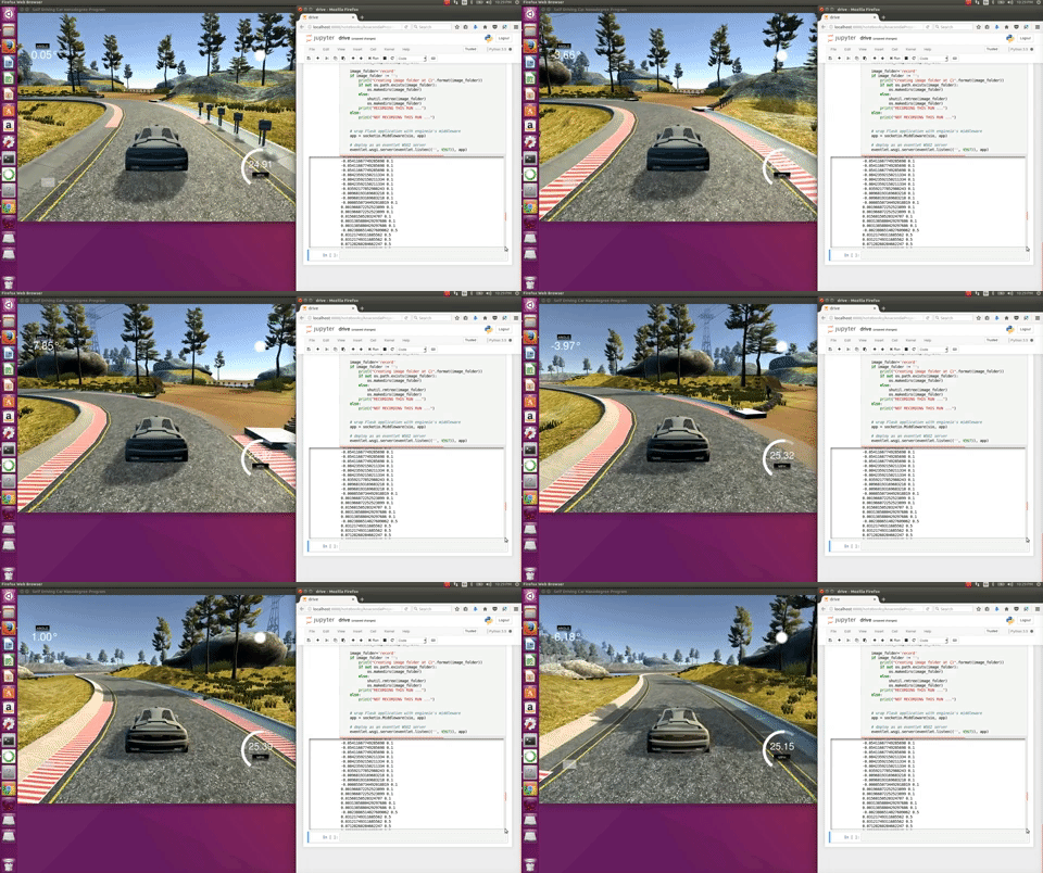
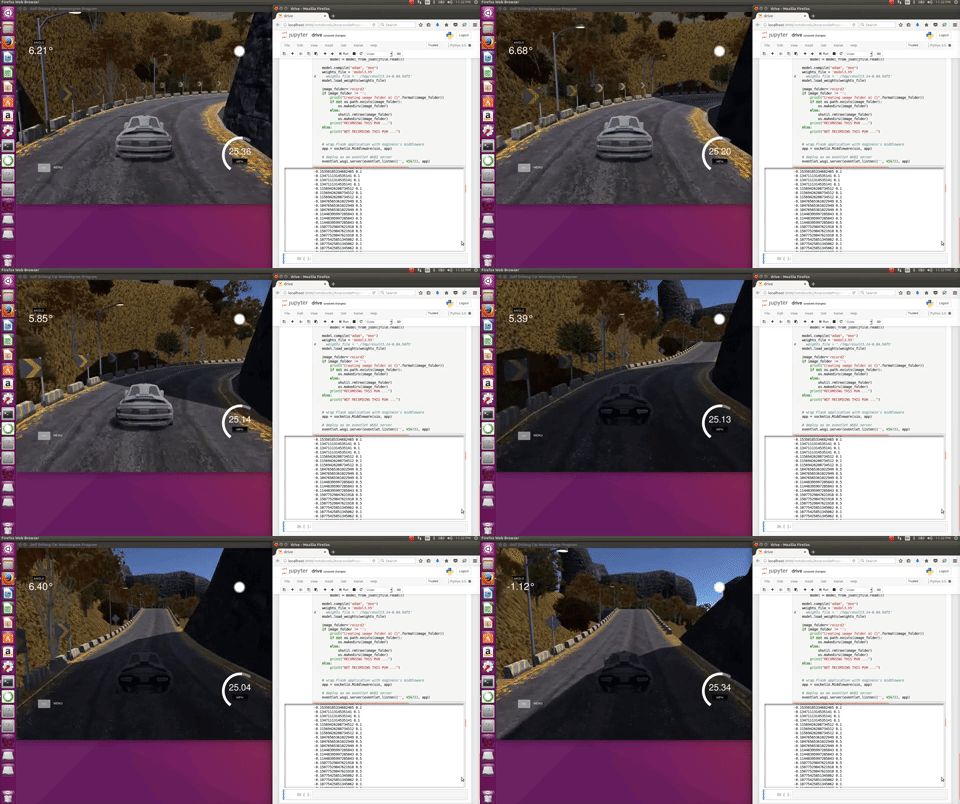
3. Simplified VGG Net - with configuration A
Discussion
After tried different network architecture – Nvidia, Comma AI and VGG-A one, the Nvidia one achieves the best cost efficient performance. Its model size is small while relatively good generalizability. This is the beauty and benefit of Transfer learning in machine learning.
The last proposed model by Dr. Junsheng Fu is derived from VGG and LeNet, which is more complex than LeNet but smaller than VGG. To avoid overfitting, he added tow dropout layers into the model and reduce the number of neurons in FC layers, which reduce both the train loss and validation loss.
The udacity dataset is already smoothed, or at least is joystick or wheeled controller input. And the model clones them. It is perfecty matched the title “behavioral clone”. If you are good driver, it clones. If you are bad driver, it clones too. However most of the time, it is hard to figure out who is better driver, human or machine.
I thought a smooth steering curve is better for the training, but it turn out not really the case. Over smoothed curve yield very aggressive turnning. Maybe it is a very good result, we just need fine tune the controller to handle it properly. Also, in the real world, most of the time, the steering wheel is in netural position. Train the machine not to over react is harder than keep moving.
20 minutes to train around 13,000 66x200 size images with GPU(GTX 980m) is not bad. It turns out that using GPU is about 4 times faster than CPU. The bottle neck seems to be how many images(batch size) GPU can process at the same time. The large batch size will consume larger GPU memory, but leads to faster training time.
Future Work
This is the self driving car future we are looking for. We need overcome some obstacles:
- Better training data
- More compute power
- Standardize Network Architecture
- Try and error approach, and engineering approach
- Working with real environment data
The simulator also provide real time steering_angle, throttle, speed and image feed. Therefore, it is possible to record new training set driving by the machine. Then train the machine again. After few generation, the machine driver will be better than human. I am going to explore more about the reinforcement learning.
The second version of simulator is out with a more challenging unseen track. It will be beneficial to generalize a model that can succefully drive in both tracks.
Reference
There are many online resources available and helpful for this project. Thank you everyone to share them to the world.
- https://github.com/JunshengFu/driving-behavioral-cloning
- https://medium.com/@mohankarthik/cloning-a-car-to-mimic-human-driving-5c2f7e8d8aff#.kot5rcn4b
- https://medium.com/@ksakmann/behavioral-cloning-make-a-car-drive-like-yourself-dc6021152713#.dttvi1ki4
- https://chatbotslife.com/learning-human-driving-behavior-using-nvidias-neural-network-model-and-image-augmentation-80399360efee#.ykemywxos
- https://github.com/upul/behavioral_cloning
- https://review.udacity.com/
- http://stackoverflow.com/questions/1756096/understanding-generators-in-python
- http://www.pyimagesearch.com/2015/10/05/opencv-gamma-correction/
- NVIDIA’s “End to End Learning for Self-Driving Cars” paper
- https://github.com/mvpcom/Udacity-CarND-Project-3
- https://github.com/karolmajek/BehavioralCloning-CarSteering
- https://github.com/commaai/research/blob/master/train_steering_model.py
- https://chatbotslife.com/using-augmentation-to-mimic-human-driving-496b569760a9
- https://github.com/vxy10/P3-BehaviorCloning
- https://github.com/ctsuu/Behavioral-Cloning
- https://github.com/ancabilloni/SDC-P3-BehavioralCloning/
- https://github.com/georgesung/behavioral_cloning
- and many many comments in slack channels.